Quickstart

This page introduces basic Pathfinder usage with examples.

A 5-dimensional multivariate normal

For a simple example, we'll run Pathfinder on a multivariate normal distribution with a dense covariance matrix. Pathfinder can take a log-density function. By default, the gradient of the log-density function is computed using ForwardDiff.

using ADTypes, ForwardDiff, LinearAlgebra, LogDensityProblems,
      Pathfinder, Printf, ReverseDiff, StatsPlots, Random
Random.seed!(42)

struct MvNormalProblem{T,S}
    μ::T  # mean
    P::S  # precision matrix
end
function (prob::MvNormalProblem)(x)
    z = x - prob.μ
    return -dot(z, prob.P, z) / 2
end

Σ = [
    2.71   0.5    0.19   0.07   1.04
    0.5    1.11  -0.08  -0.17  -0.08
    0.19  -0.08   0.26   0.07  -0.7
    0.07  -0.17   0.07   0.11  -0.21
    1.04  -0.08  -0.7   -0.21   8.65
]
μ = [-0.55, 0.49, -0.76, 0.25, 0.94]
P = inv(Symmetric(Σ))
prob_mvnormal = MvNormalProblem(μ, P)

Now we run pathfinder.

result = pathfinder(prob_mvnormal; dim=5, init_scale=4)

Single-path Pathfinder result
  tries: 1
  draws: 5
  fit iteration: 5 (total: 5)
  fit ELBO: 3.84 ± 0.0
  fit distribution: Distributions.MvNormal{Float64, Pathfinder.WoodburyPDMat{Float64, LinearAlgebra.Diagonal{Float64, Vector{Float64}}, Matrix{Float64}, Matrix{Float64}, Pathfinder.WoodburyPDFactorization{Float64, LinearAlgebra.Diagonal{Float64, Vector{Float64}}, LinearAlgebra.QRCompactWYQ{Float64, Matrix{Float64}, Matrix{Float64}}, LinearAlgebra.UpperTriangular{Float64, Matrix{Float64}}}}, Vector{Float64}}(
dim: 5
μ: [-0.55, 0.49, -0.76, 0.25, 0.94]
Σ: [2.709999999999999 0.5000000000000003 … 0.07000000000000016 1.0399999999999996; 0.5000000000000003 1.1100000000000012 … -0.17000000000000046 -0.07999999999999952; … ; 0.07000000000000016 -0.17000000000000046 … 0.10999999999999943 -0.21000000000000008; 1.0399999999999996 -0.07999999999999952 … -0.21000000000000008 8.649999999999997]
)

result is a PathfinderResult. See its docstring for a description of its fields.

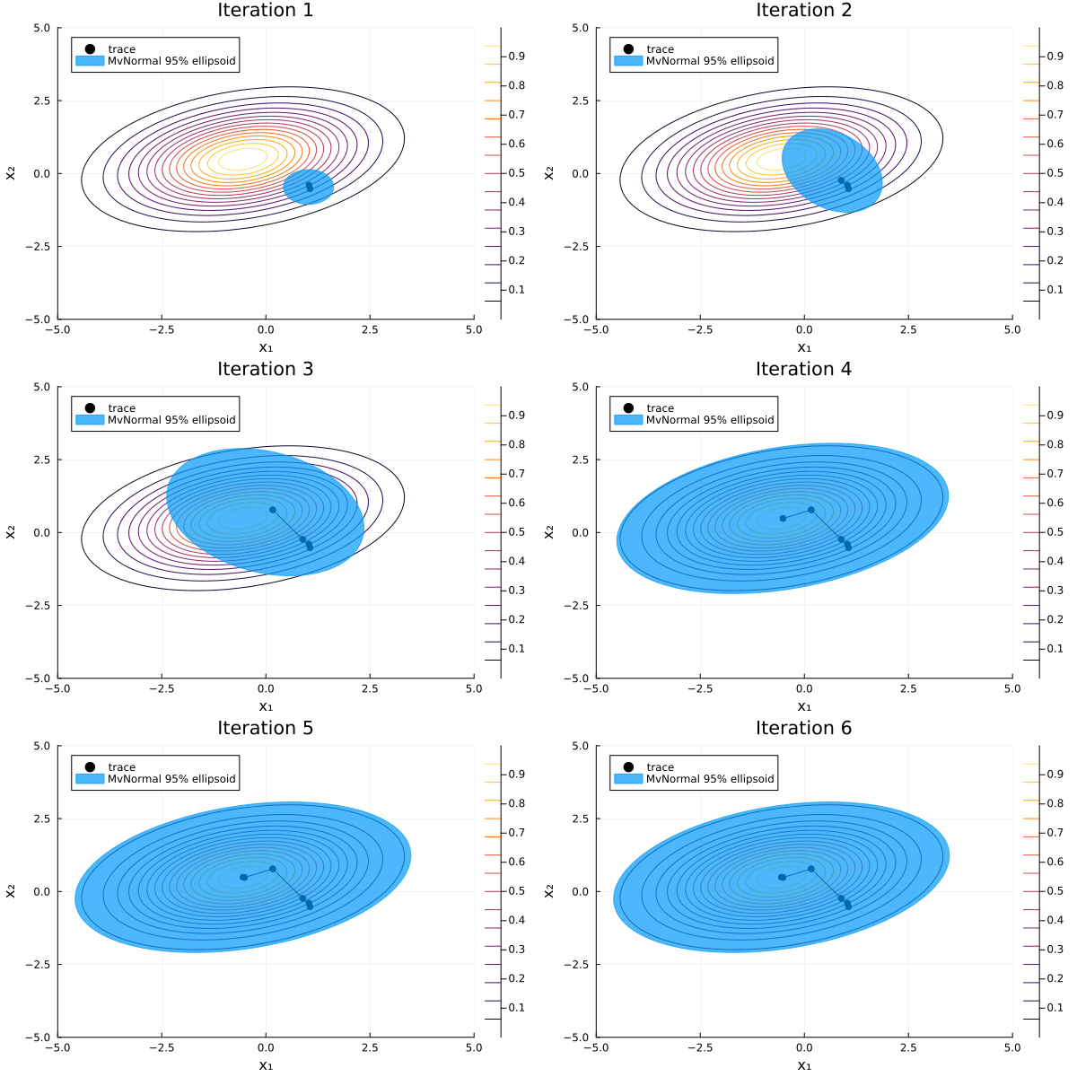
The L-BFGS optimizer constructs an approximation to the inverse Hessian of the negative log density using the limited history of previous points and gradients. For each iteration, Pathfinder uses this estimate as an approximation to the covariance matrix of a multivariate normal that approximates the target distribution. The distribution that maximizes the evidence lower bound (ELBO) is stored in result.fit_distribution. Its mean and covariance are quite close to our target distribution's.

result.fit_distribution.μ

5-element Vector{Float64}:
 -0.55
  0.49
 -0.76
  0.25
  0.94

result.fit_distribution.Σ

5×5 Pathfinder.WoodburyPDMat{Float64, LinearAlgebra.Diagonal{Float64, Vector{Float64}}, Matrix{Float64}, Matrix{Float64}, Pathfinder.WoodburyPDFactorization{Float64, LinearAlgebra.Diagonal{Float64, Vector{Float64}}, LinearAlgebra.QRCompactWYQ{Float64, Matrix{Float64}, Matrix{Float64}}, LinearAlgebra.UpperTriangular{Float64, Matrix{Float64}}}}:
 2.71   0.5    0.19   0.07   1.04
 0.5    1.11  -0.08  -0.17  -0.08
 0.19  -0.08   0.26   0.07  -0.7
 0.07  -0.17   0.07   0.11  -0.21
 1.04  -0.08  -0.7   -0.21   8.65

result.draws is a Matrix whose columns are the requested draws from result.fit_distribution:

result.draws

5×5 Matrix{Float64}:
 -0.275857  -1.38317   -0.584716    0.600188  -2.56678
  0.558877  -0.471967   1.22294     1.48115    0.478595
 -0.537484  -0.140841  -1.03717    -0.958389  -1.33453
  0.433044   0.414753   0.0817292   0.184138  -0.31791
 -2.98036    5.16025   -1.42753    -0.30277    3.03684

We can visualize Pathfinder's sequence of multivariate-normal approximations with the following function:

function plot_pathfinder_trace(
    result, logp_marginal, xrange, yrange, maxiters;
    show_elbo=false, flipxy=false, kwargs...,
)
    iterations = min(length(result.optim_trace) - 1, maxiters)
    trace_points = result.optim_trace.points
    trace_dists = result.fit_distributions
    anim = @animate for i in 1:iterations
        contour(xrange, yrange, exp ∘ logp_marginal ∘ Base.vect; label="")
        trace = trace_points[1:(i + 1)]
        dist = trace_dists[i + 1]
        plot!(
            first.(trace), getindex.(trace, 2);
            seriestype=:scatterpath, color=:black, msw=0, label="trace",
        )
        covellipse!(
            dist.μ[1:2], dist.Σ[1:2, 1:2];
            n_std=2.45, alpha=0.7, color=1, linecolor=1, label="MvNormal 95% ellipsoid",
        )
        title = "Iteration $i"
        if show_elbo
            est = result.elbo_estimates[i]
            title *= "  ELBO estimate: " * @sprintf("%.1f", est.value)
        end
        plot!(; xlims=extrema(xrange), ylims=extrema(yrange), title, kwargs...)
    end
    return anim
end;

xrange = -5:0.1:5
yrange = -5:0.1:5

μ_marginal = μ[1:2]
P_marginal = inv(Σ[1:2,1:2])
logp_mvnormal_marginal(x) = -dot(x - μ_marginal, P_marginal, x - μ_marginal) / 2

anim = plot_pathfinder_trace(
    result, logp_mvnormal_marginal, xrange, yrange, 20;
    xlabel="x₁", ylabel="x₂",
)
gif(anim; fps=5)

A banana-shaped distribution

Now we will run Pathfinder on the following banana-shaped distribution with density

\[\pi(x_1, x_2) = e^{-x_1^2 / 2} e^{-5 (x_2 - x_1^2)^2 / 2}.\]

Pathfinder can also take any object that implements the LogDensityProblems interface interface. This can also be used to manually define the gradient of the log-density function.

First we define the log density problem:

Random.seed!(23)

struct BananaProblem end
function LogDensityProblems.capabilities(::Type{<:BananaProblem})
    return LogDensityProblems.LogDensityOrder{1}()
end
LogDensityProblems.dimension(::BananaProblem) = 2
function LogDensityProblems.logdensity(::BananaProblem, x)
    return -(x[1]^2 + 5(x[2] - x[1]^2)^2) / 2
end
function LogDensityProblems.logdensity_and_gradient(::BananaProblem, x)
    a = (x[2] - x[1]^2)
    lp = -(x[1]^2 + 5a^2) / 2
    grad_lp = [(10a - 1) * x[1], -5a]
    return lp, grad_lp
end

prob_banana = BananaProblem()

and then visualise it:

xrange = -3.5:0.05:3.5
yrange = -3:0.05:7
logp_banana(x) = LogDensityProblems.logdensity(prob_banana, x)
contour(xrange, yrange, exp ∘ logp_banana ∘ Base.vect; xlabel="x₁", ylabel="x₂")

Now we run pathfinder.

result = pathfinder(prob_banana; init_scale=10)

Single-path Pathfinder result
  tries: 1
  draws: 5
  fit iteration: 10 (total: 17)
  fit ELBO: 0.77 ± 0.12
  fit distribution: Distributions.MvNormal{Float64, Pathfinder.WoodburyPDMat{Float64, LinearAlgebra.Diagonal{Float64, Vector{Float64}}, Matrix{Float64}, Matrix{Float64}, Pathfinder.WoodburyPDFactorization{Float64, LinearAlgebra.Diagonal{Float64, Vector{Float64}}, LinearAlgebra.QRCompactWYQ{Float64, Matrix{Float64}, Matrix{Float64}}, LinearAlgebra.UpperTriangular{Float64, Matrix{Float64}}}}, Vector{Float64}}(
dim: 2
μ: [0.08620518601715449, -0.12005910142708787]
Σ: [0.7477323503101031 0.6844011151001731; 0.6844011151001731 0.8382052638654003]
)

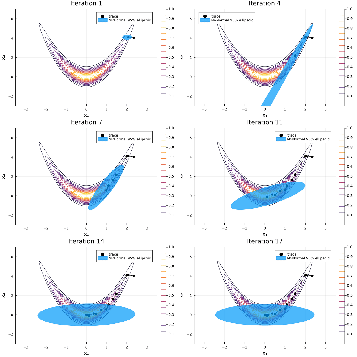
As before we can visualise each iteration of the algorithm.

anim = plot_pathfinder_trace(
    result, logp_banana, xrange, yrange, 20;
    xlabel="x₁", ylabel="x₂",
)
gif(anim; fps=5)

Since the distribution is far from normal, Pathfinder is unable to fit the distribution well. Especially for such complicated target distributions, it's always a good idea to run multipathfinder, which runs single-path Pathfinder multiple times.

ndraws = 1_000
result = multipathfinder(prob_banana, ndraws; nruns=20, init_scale=10)

Multi-path Pathfinder result
  runs: 20
  draws: 1000
  Pareto shape diagnostic: 0.5 (good)

result is a MultiPathfinderResult. See its docstring for a description of its fields.

result.fit_distribution is a uniformly-weighted Distributions.MixtureModel. Each component is the result of a single Pathfinder run. It's possible that some runs fit the target distribution much better than others, so instead of just drawing samples from result.fit_distribution, multipathfinder draws many samples from each component and then uses Pareto-smoothed importance resampling (using PSIS.jl) from these draws to better target prob_banana.

The Pareto shape diagnostic informs us on the quality of these draws. Here the Pareto shape $k$ diagnostic is bad ($k > 0.7$), which tells us that these draws are unsuitable for computing posterior estimates, so we should definitely run MCMC to get better draws. Still, visualizing the draws can still be useful.

x₁_approx = result.draws[1, :]
x₂_approx = result.draws[2, :]

contour(xrange, yrange, exp ∘ logp_banana ∘ Base.vect)
scatter!(x₁_approx, x₂_approx; msw=0, ms=2, alpha=0.5, color=1)
plot!(xlims=extrema(xrange), ylims=extrema(yrange), xlabel="x₁", ylabel="x₂", legend=false)

While the draws do a poor job of covering the tails of the distribution, they are still useful for identifying the nonlinear correlation between these two parameters.

A 100-dimensional funnel

As we have seen above, running multi-path Pathfinder is much more useful for target distributions that are far from normal. One particularly difficult distribution to sample is Neal's funnel:

\[\begin{aligned} \tau &\sim \mathrm{Normal}(\mu=0, \sigma=3)\\ \beta_i &\sim \mathrm{Normal}(\mu=0, \sigma=e^{\tau/2}) \end{aligned}\]

Such funnel geometries appear in other models (e.g. many hierarchical models) and typically frustrate MCMC sampling. Multi-path Pathfinder can't sample the funnel well, but it can quickly give us draws that can help us diagnose that we have a funnel.

In this example, we draw from a 100-dimensional funnel and visualize 2 dimensions.

using ReverseDiff, ADTypes

Random.seed!(68)

function logp_funnel(x)
    n = length(x)
    τ = x[1]
    β = view(x, 2:n)
    return ((τ / 3)^2 + (n - 1) * τ + sum(b -> abs2(b * exp(-τ / 2)), β)) / -2
end

First, let's fit this posterior with single-path Pathfinder. For high-dimensional problems, it's better to use reverse-mode automatic differentiation. Here, we'll use ADTypes.AutoReverseDiff to specify that ReverseDiff.jl should be used.

result_single = pathfinder(logp_funnel; dim=100, init_scale=10, adtype=AutoReverseDiff())

Single-path Pathfinder result
  tries: 1
  draws: 5
  fit iteration: 11 (total: 51)
  fit ELBO: 86.83 ± 1.68
  fit distribution: Distributions.MvNormal{Float64, Pathfinder.WoodburyPDMat{Float64, LinearAlgebra.Diagonal{Float64, Vector{Float64}}, Matrix{Float64}, Matrix{Float64}, Pathfinder.WoodburyPDFactorization{Float64, LinearAlgebra.Diagonal{Float64, Vector{Float64}}, LinearAlgebra.QRCompactWYQ{Float64, Matrix{Float64}, Matrix{Float64}}, LinearAlgebra.UpperTriangular{Float64, Matrix{Float64}}}}, Vector{Float64}}(
dim: 100
μ: [-0.9264005866387869, 0.07440420104538821, 0.3463222620020974, 0.1744876663432293, -0.36311345688024765, 0.29524861072520275, 0.056618694713401876, 0.3492313184188715, 0.12947288324963313, 0.16483909485180306  …  -0.10556400229650764, -0.024869129620949795, -0.11003557294663188, -0.1565057244546378, 0.33271287862572607, -0.04300991530903499, 0.0036211670995282908, 0.10988664138021828, -0.11817685635919295, -0.035731556478309494]
Σ: [0.01367138121749178 -0.0010832703878637937 … 0.0017205473272006485 0.0005202283664656283; -0.0010832703878637937 0.4421982187095132 … 0.00017348838114317279 4.539664260241101e-5; … ; 0.0017205473272006485 0.00017348838114317279 … 0.447939864191428 -7.951274026910362e-5; 0.0005202283664656283 4.539664260241101e-5 … -7.951274026910362e-5 0.4392274346299829]
)

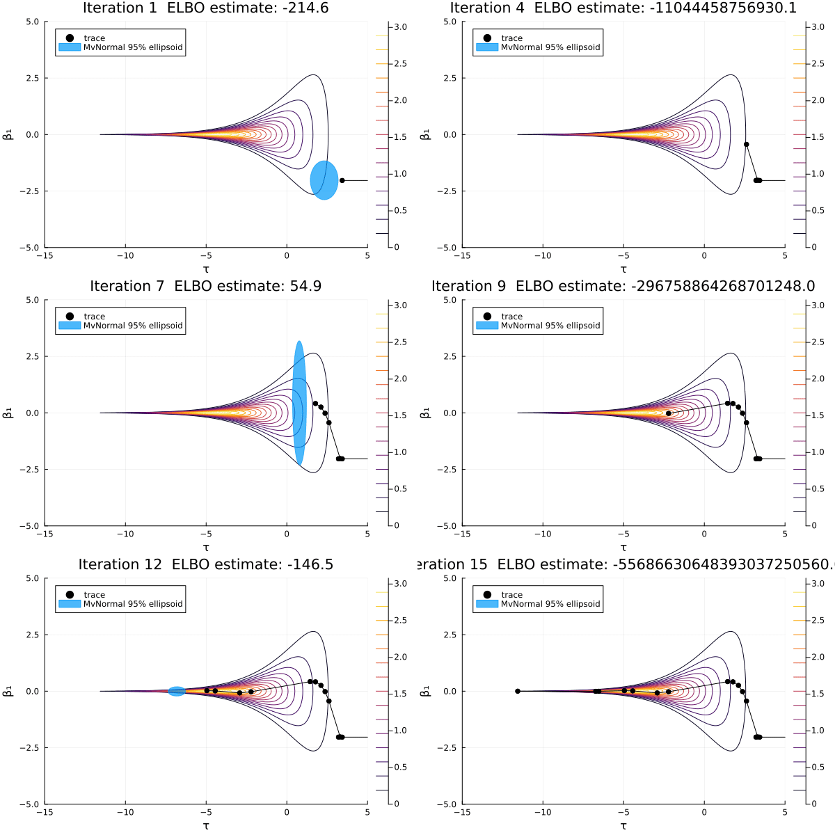
Let's visualize this sequence of multivariate normals for the first two dimensions.

β₁_range = -5:0.01:5
τ_range = -15:0.01:5

anim = plot_pathfinder_trace(
    result_single, logp_funnel, τ_range, β₁_range, 15;
    show_elbo=true, xlabel="τ", ylabel="β₁",
)
gif(anim; fps=2)

For this challenging posterior, we can again see that most of the approximations are not great, because this distribution is not normal. Also, this distribution has a pole instead of a mode, so there is no MAP estimate, and no Laplace approximation exists. As optimization proceeds, the approximation goes from very bad to less bad and finally extremely bad. The ELBO-maximizing distribution is at the neck of the funnel, which would be a good location to initialize MCMC.

Now we run multipathfinder.

ndraws = 1_000
result = multipathfinder(logp_funnel, ndraws; dim=100, nruns=20, init_scale=10, adtype=AutoReverseDiff())

Multi-path Pathfinder result
  runs: 20
  draws: 1000
  Pareto shape diagnostic: 0.93 (bad)

Again, the poor Pareto shape diagnostic indicates we should run MCMC to get draws suitable for computing posterior estimates.

We can see that the bulk of Pathfinder's draws come from the neck of the funnel, where the fit from the single path we examined was located.

τ_approx = result.draws[1, :]
β₁_approx = result.draws[2, :]

contour(τ_range, β₁_range, exp ∘ logp_funnel ∘ Base.vect)
scatter!(τ_approx, β₁_approx; msw=0, ms=2, alpha=0.5, color=1)
plot!(; xlims=extrema(τ_range), ylims=extrema(β₁_range), xlabel="τ", ylabel="β₁", legend=false)